Detecting adaptation in very structured populations: how hard can it be?

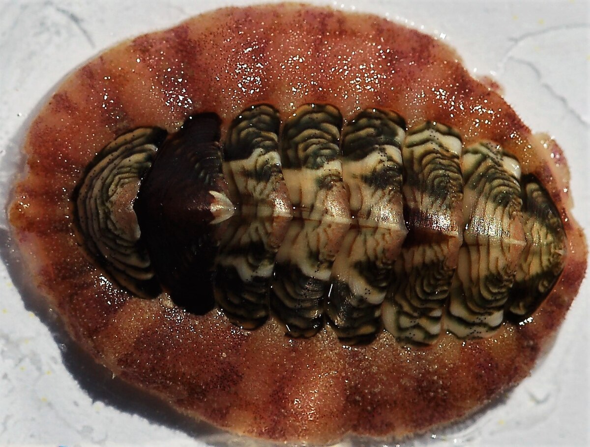
I’m very happy to let you know that a new paper from the PhD thesis of Priscila Salloum is now out (in early view) in Journal of Animal Ecology! The idea of Priscila’s thesis (at the University of Auckland, co-directed by Shane Lavery and Anna Santure and, well, myself) was to use genomics and morphometrics data to characterise and understand the distribution of the diversity in a New Zealand marine mollusc, which she chose to be the beautiful Onithochiton neglectus.

Priscila previously analysed genetic markers to show that this species has a weird population structure: populations from the North Island of New Zealand, that are geographically closer are very distant genetically speaking and populations from the South Island, Chatham Island and Sub-Antarctic Islands are much more similar, genetically speaking.

Generally, we observe that genetic differentiation follows geographic distances, simply because populations that are further apart tend to exchange less migrants. So what is going on here?

Well, this is in fact well explained by the fact that this chiton species is able to “kelp-raft” on the algae species Durvillea antarctica. By doing so, species from the Sub-Antarctic Islands are, in fact, more “connected” through big oceanic currents than are the geographically closer Northern populations that are more isolated, especially due to local loops in the currents.

OK, now, on to the question at hand, and why this previous context matters, we wanted to detect local adaptation, what is that? Local adaptation happens when different populations of a species are subject to differences in their local environment, generating differential selection among populations. If the correct conditions are met, then populations will change in their genetic composition to respond to this local selection, which means by definition that they adapt! Well, this is what we call “local adaptation”. And in theory, it should be possible to detect locations within the genome (a.k.a. loci) that are involved in this local adaptation. To do so, there are two main options : detecting loci that are especially differentiated between populations (more than the rest of the genome) because they responded to selection or trying to correlate the frequencies of the variants at each loci with some environmental variable.

This is all very well, but what about this “population structure” stuff then? Well, imagine that you want to find genes linked with the colour of the eyes, one way you could do it is study a group with blue eyes, and another group with brown eyes, and any genetic variation that is strongly linked with belonging within the blue or brown eyes group must be linked to eye colouration right? Well, maybe, but what if your “blue eye group” is composed of Swedish people and your “brown eye group” is composed of Japanese people? Surely, and although ethnic groups share a huge lot of their genome of course, there are quite a few loci in the genome that would differ between groups of Swedish and Japanese people without having any link whatsoever with eye colouration! So concluding that they influence eye colouration would be what we call a false positive.This is why, when looking for genetic association with phenotypic characteristics like this, or when looking for signals of selection within the genome, we account for “population structure”, i.e. the fact that individuals do not belong to the same, homogenous group, but to differentiated groups (within or among populations, depending on context).

Thing is, I’ve shown a while ago that genome scan methods to detect selection suffer from a very strong issue of false positives when exposed to strong population structure even when they are supposed to correct to said population structure (to put it shortly, it’s something easier said than done!). And thus, when we faced this problem in the real world with this chiton species with strong and distinguishable populations, we used three different approaches to decrease the proportion of false positives among our positive results. The first approach was very simple: we distinguished between the extremely differentiated Northern populations and the less differentiation Southern ones. The second was about simulating random environmental variable. If loci are often significantly associated with a perfectly arbitrary variable that only exists because it comes from a computer program, surely, the fact that it is associated with a “real” environmental variable must be regarded with suspicion. It certainly does not mean the locus is not subjected to selection (it certainly could be!), only that our statistical test was, basically, not informative at all!

The third approach was about using several methods and combining their results. I’ve shown in the above study that combining methods helps enrich our set of positive loci for true, rather than false, positives. But using the intersection of methods as I used then (all methods have to agree about a positive being positive) is a very strict thing which I never grew satisfied with. A possible solution would be to compute a kind of average between the methods… But using arithmetic mean is also very unsatisfying, as it provides a lot of weight for non-positive tests (just as using the harmonic mean would favour positive tests). Then, possibly, the geometric mean (the most balanced of all three) would hit the right spot? A more technical (sorry…) argument in favour of the geometric mean is that it can be seen as taking the average on the log-scale (by that I mean taking the logarithm of our variable and work with these new values), which happens to be a very good scale to interpret significance testing (stuff like p- or q-values). Although I checked the behaviour of this on old simulations, I’d like to properly tackle this idea with a dedicated simulation study!

So, we implemented all of these layers of refinement, in order to decrease any issues with false positives and we managed to go from hundreds or even thousands of markers that could have been considered as positives to only 86. Of course, in doing so, we most certainly threw out some interesting “truly positive” loci. But life is such that there is a no way (by definition…) to distinguish a false from a true positive (except testing everything experimentally!), and the only thing we can do is enrich our set of positive loci for true positives respective to the false positives. This is what our filter layers aimed to do, but clearly, we still need even better methods to tackle this very prevalent problem!